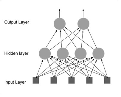
What is Neural Network? why to choose neural network projects using matlab?
NEURAL NETWORK MATLAB is a powerful technique which is used to solve many real world problems. Information processing paradigm in neural network Matlab projects is inspired by biological nervous systems. NEURAL NETWORK MATLAB is used to perform specific applications as pattern recognition or data classification. Ability to deal with incomplete information is main advantage in neural network projects.
- Completed Neural Network Matlab Projects 52%
- On going Neural Network Matlab Projects 19%

Advantages of Neural Networks using Matlab :
- Graceful Degradation.
- Rules are implicit rather than explicit.
- More like a real nervous system.
Applications of Neural Networks Matlab Projects:
- Pattern Recognition.
- Control Systems & Monitoring.
- Forecasting.
- Mobile Computing.
- Investment Analysis.
- Marketing and Financial .
Types of Neural Network Algorithms:
- Multi-Layer Perceptron (MLP).
- Radial Basis Function (RBF).
- Learning Vector Quantization (LVQ).
Multi-Layer Perceptron:
- MLP is used to describe any general feed forward network.
- Back propagation algorithm which is used to train it.
Code for MLP:
% XOR input for x1 and x2
input = [0 0; 0 1; 1 0; 1 1];
% Desired output of XOR
output = [0;1;1;0];
% Initialize the bias
bias = [-1 -1 -1];
% Learning coefficient
coeff = 0.7;
% Number of learning iterations
iterations = 10000;
% Calculate weights randomly using seed.
rand(‘state’,sum(100*clock));
weights = -1 +2.*rand(3,3);
for i = 1:iterations
out = zeros(4,1);
numIn = length (input(:,1));
for j = 1:numIn
% Hidden layer
H1 = bias(1,1)*weights(1,1)
+ input(j,1)*weights(1,2)
+ input(j,2)*weights(1,3);
% Send data through sigmoid function 1/1+e^-x
% Note that sigma is a different m file
% that I created to run this operation
x2(1) = sigma(H1);
H2 = bias(1,2)*weights(2,1)
+ input(j,1)*weights(2,2)
+ input(j,2)*weights(2,3);
x2(2) = sigma(H2);
% Output layer
x3_1 = bias(1,3)*weights(3,1)
+ x2(1)*weights(3,2)
+ x2(2)*weights(3,3);
out(j) = sigma(x3_1);
% Adjust delta values of weights
% For output layer:
% delta(wi) = xi*delta,
% delta = (1-actual output)*(desired output – actual output)
delta3_1 = out(j)*(1-out(j))*(output(j)-out(j));
% Propagate the delta backwards into hidden layers
delta2_1 = x2(1)*(1-x2(1))*weights(3,2)*delta3_1;
delta2_2 = x2(2)*(1-x2(2))*weights(3,3)*delta3_1;
% Add weight changes to original weights
% And use the new weights to repeat process.
% delta weight = coeff*x*delta
for k = 1:3
if k == 1 % Bias cases
weights(1,k) = weights(1,k) + coeff*bias(1,1)*delta2_1;
weights(2,k) = weights(2,k) + coeff*bias(1,2)*delta2_2;
weights(3,k) = weights(3,k) + coeff*bias(1,3)*delta3_1;
else % When k=2 or 3 input cases to neurons
weights(1,k) = weights(1,k) + coeff*input(j,1)*delta2_1;
weights(2,k) = weights(2,k) + coeff*input(j,2)*delta2_2;
weights(3,k) = weights(3,k) + coeff*x2(k-1)*delta3_1;
end
end
end
Radial Basis Function:
- Use of multidimensional surface to interpolate the test data.
- Design of NN as curve fitting problem.
Code for RDF
%Matlab code for Radial Basis Functions
clc;x=-1:0.05:1;
%generating training data with Random Noise
fori=1:length(x)
y(i)=1.2*sin(pi*x(i))-cos(2.4*pi*x(i))+0.3*randn;
end
% Framing the interpolation matrix for training data
t=length(x);
fori=1:1:t
forj=1:1:t
h=x(i)-x(j); k=h^2/.02;
train(i,j)=exp(-k);
end
end
W=inv(train)*y’;
% Testing the trained RBF
xtest=-1:0.01:1;
%ytest is the desired output
ytest=1.2*sin(pi*xtest)-cos(2.4*pi*xtest);
% Framing the interpolation matrix for test data
t=length(x);
fori=1:1:t
forj=1:1:t
h=x(i)-x(j); k=h^2/.02;
train(i,j)=exp(-k);
end
end
W=inv(train)*y’;
% Testing the trained RBF
xtest=-1:0.01:1;
%ytest is the desired output
ytest=1.2*sin(pi*xtest)-cos(2.4*pi*xtest);
% Framing the interpolation matrix for test data
t1=length(xtest);
t=length(x);
fori=1:1:t1
forj=1:1:t
h=xtest(i)-x(j);
k=h^2/.02;
test(i,j)=exp(-k);
end
end
actual_test=test*W;
% Plotting the Performance of the network
figure;
plot(xtest,ytest,’b-‘,xtest,actual_test,’r+’);
xlabel(‘Xtest value’);
ylabel(‘Ytest value’);
h = legend(‘Desired output’,’Approximated curve’,2);
set(h);
LVQ:
- Learning vector quantization is a supervised technique which have labeled input data.
- To improve quality of the classifier decision regions.
- Goal of self-organizing map is to perform transformation.
Sample Code for LVQ:
Classes are transformed to vectors it can be treated as target
t = ind2vec(c);
LVQ network represents clusters of vectors with hidden neurons, and groups the clusters with output neurons to form the desired classes
colormap(hsv);
plotvec(x,c)
title(‘Input Vectors’);
xlabel(‘x(1)’);
ylabel(‘x(2)’);
network is then configured for inputs X and targets T
net = lvqnet(4,0.1);
net = configure(net,x,t);
Train the network:
net.trainParam.epochs=150;
net=train(net,x,t);
cla;
plotvec(x,c);
hold on;
plotvec(net.IW{1}’,vec2ind(net.LW{2}),’o’);


